

In this article, we'll use Data Science and Machine Learning tools to analyze data from a house prices dataset.
We will begin by performing Exploratory Data Analysis on the data. We'll create a script to clean the data, then we will use the cleaned data to create a Machine Learning Model. Finally we use the Machine Learning model to implement our own prediction API.
The full source code is in the GitHub repository with clear instructions to execute this end-to-end project.
Quick info: You can download a PDF version of this Data Science and Machine Learning Project with the full source code repository linked in the book.
Ready to dive in?
Table of contents
- Github Repository
- EDA (Exploratory Data Analysis)
- Data Cleaning Script
- Machine Learning Model
- API
- Conclusion
Github Repository
You can download the complete code in the Github Repository.
In the repository you will find:
- requirements.txt: The packages you need to install using pip
- raw_data.csv: The raw data we are using on this project
- Exploratory-Data-Analysis-House-Prices.ipynb: The Jupyter Notebook with the Exploratory Data Analysis
- data_cleaning.py: The script that cleans the data
- train_model.py: The script to train the Machine Learning Model using the cleaned data
- predict.py: The file with the HousePriceModel class that we use to load the ML model and make the predictions
- api.py: The API created with the framework FastAPI
- test_api.py: The script to test the API
To use the data and code in the repository, follow the steps in the next sections.
Environment and Packages
Create a virtual environment to isolate your Python project:
python3 -m venv venv
Activate the virtual environment like this:
source ./venv/bin/activate
And then install the necessary packages:
pip install -r requirements.txt
You should see a message similar to this at the end:
Successfully installed Babel-2.9.0 Jinja2-2.11.3 MarkupSafe-1.1.1 Pygments-2.8.0 Send2Trash-1.5.0 anyio-2.1.0 argon2-cffi-20.1.0 async-generator-1.10 attrs-20.3.0 backcall-0.2.0 bleach-3.3.0 certifi-2020.12.5 cffi-1.14.5 chardet-4.0.0 click-7.1.2 decorator-4.4.2 defusedxml-0.6.0 entrypoints-0.3 fastapi-0.63.0 h11-0.12.0 idna-2.10 ipykernel-5.4.3 ipython-7.20.0 ipython-genutils-0.2.0 jedi-0.18.0 joblib-1.0.1 json5-0.9.5 jsonschema-3.2.0 jupyter-client-6.1.11 jupyter-core-4.7.1 jupyter-server-1.3.0 jupyterlab-3.0.7 jupyterlab-pygments-0.1.2 jupyterlab-server-2.2.0 mistune-0.8.4 nbclassic-0.2.6 nbclient-0.5.2 nbconvert-6.0.7 nbformat-5.1.2 nest-asyncio-1.5.1 notebook-6.2.0 numpy-1.20.1 packaging-20.9 pandas-1.2.2 pandocfilters-1.4.3 parso-0.8.1 pexpect-4.8.0 pickleshare-0.7.5 prometheus-client-0.9.0 prompt-toolkit-3.0.16 ptyprocess-0.7.0 pycparser-2.20 pydantic-1.7.3 pyparsing-2.4.7 pyrsistent-0.17.3 python-dateutil-2.8.1 pytz-2021.1 pyzmq-22.0.3 requests-2.25.1 scikit-learn-0.24.1 scipy-1.6.0 six-1.15.0 sniffio-1.2.0 starlette-0.13.6 terminado-0.9.2 testpath-0.4.4 threadpoolctl-2.1.0 tornado-6.1 traitlets-5.0.5 urllib3-1.26.3 uvicorn-0.13.3 wcwidth-0.2.5 webencodings-0.5.1
EDA (Exploratory Data Analisys)
To check out the EDA (Exploratory Data Analisys):
jupyter-notebook Exploratory-Data-Analysis-House-Prices.ipynb
Then, with the Jupyter Notebook open, go to Cell > Run All to run all the commands.
Then execute the following steps in this sequence.
Clean the Data
To perform the cleaning process on the raw data, type the following command:
python data_cleaning.py
Here's the expected output:
Original Data: (1168, 81)
Columns with missing values: 0
Series([], dtype: int64)
After Cleaning: (1168, 73)
This will generate the 'cleaned_data.csv'.
Create the Machine Learning Model
To train the model, enter this command:
python train_model.py
Here's the expected output:
Train data for modeling: (934, 73)
Test data for predictions: (234, 73)
Training the model ...
Testing the model ...
Average Price Test: 175652.0128205128
RMSE: 11098.009355519898
Model saved at model.pkl
This will create the 'train.csv', 'test.csv', and 'model.pkl'.
Run and test the API
To run the API, type this command:
uvicorn api:app
Here's the expected output:
INFO:     Started server process [56652]
INFO:     Waiting for application startup.
INFO:     Application startup complete.
INFO:     Uvicorn running on http://127.0.0.1:8000 (Press CTRL+C to quit)
To test the API, on another terminal activate the virtual environment again (this time you already have the packages installed):
source ./venv/bin/activate
And then run:
python test_api.py
Here's the expected output:
The actual Sale Price: 109000
The predicted Sale Price: 109000.01144237864
Exploratory Data Analysis
Let's begin with an Exploratory Data Analysis, a.k.a EDA, of the dataset "House Prices: Advanced Regression Techniques".
We will:
- Understand the problem
- Explore the data and deal with missing values
- Select and transform variables, especially categorical ones
The Problem
This is the description of the problem on Kaggle:
"Ask a home buyer to describe their dream house, and they probably won't begin with the height of the basement ceiling or the proximity to an east-west railroad. But this playground competition's dataset proves that much more influences price negotiations than the number of bedrooms or a white-picket fence.
With 79 explanatory variables describing (almost) every aspect of residential homes in Ames, Iowa, this competition challenges you to predict the final price of each home."
So, we are going to explore the dataset, try to get some insights from it, and use some tools to transform the data into formats that make more sense.
Initial Exploration and First Insights
In this section, we are going to make an initial exploration of the dataset.
This EDA was performed on a Jupyter Notebook.
Importing Libraries
We begin by importing the libs we are going to use:
- The standard math module provides access to the mathematical functions.
- The NumPy lib is fundamental for any kind of scientific computing with Python.
- pandas is a must-have tool for data analysis and manipulation.
- matplotlib is the most complete package in Python when it comes to data visualizations.
- seaborn is based on matplotlib as a higher-level set of visualization tools, not as powerful as matplotlib, but much easier to work with and delivers a lot with less work.
import math
import numpy as np
import pandas as pd
import seaborn as sns
import matplotlib as mpl
import matplotlib.pyplot as plt

%matplotlib inline
Loading Data
Since we have tabular data, we are going to use pandas to load the data and take a first look at it.
To load the data, since the format is CSV (Comma-Separated Values), we use the read_csv() function from pandas.
Then we print its shape, which is 1168x81, meaning we have 1168 rows (records) and 81 columns (features).
Actually, we have 1169 rows in the CSV file, but the header that describes the columns doesn't count.
And we actually have 79 features since one of the columns is SalePrice, which is the column we will try to predict in a model, and we also will not use the column Id and will get rid of it later.
train = pd.read_csv('raw_data.csv')
train.shape
(1168, 81)
Looking at the Data
First, I recommend you to read this brief description of each column.
Using the head() function from pandas with an argument of 3, we can take a look at the first 3 records.
The .T means Transpose, this way we visualize rows as columns and vice-versa.
Notice how it doesn't show all of the columns in the middle and only displays ... because there are too many of them.
train.head(3).T
| 0 | 1 | 2 | |
|---|---|---|---|
| Id | 893 | 1106 | 414 |
| MSSubClass | 20 | 60 | 30 |
| MSZoning | RL | RL | RM |
| LotFrontage | 70 | 98 | 56 |
| LotArea | 8414 | 12256 | 8960 |
| ... | ... | ... | ... |
| MoSold | 2 | 4 | 3 |
| YrSold | 2006 | 2010 | 2010 |
| SaleType | WD | WD | WD |
| SaleCondition | Normal | Normal | Normal |
| SalePrice | 154500 | 325000 | 115000 |
81 rows × 3 columns
The info() method from pandas will give you a summary of the data.
Notice how Alley has 70 non-null values, meaning it doesn't have a value for most of the 1168 records.
We can also visualize the data types.
train.info()
    <class 'pandas.core.frame.DataFrame'>
    RangeIndex: 1168 entries, 0 to 1167
    Data columns (total 81 columns):
    Id               1168 non-null int64
    MSSubClass       1168 non-null int64
    MSZoning         1168 non-null object
    LotFrontage      964 non-null float64
    LotArea          1168 non-null int64
    Street           1168 non-null object
    Alley            70 non-null object
    LotShape         1168 non-null object
    LandContour      1168 non-null object
    Utilities        1168 non-null object
    LotConfig        1168 non-null object
    LandSlope        1168 non-null object
    Neighborhood     1168 non-null object
    Condition1       1168 non-null object
    Condition2       1168 non-null object
    BldgType         1168 non-null object
    HouseStyle       1168 non-null object
    OverallQual      1168 non-null int64
    OverallCond      1168 non-null int64
    YearBuilt        1168 non-null int64
    YearRemodAdd     1168 non-null int64
    RoofStyle        1168 non-null object
    RoofMatl         1168 non-null object
    Exterior1st      1168 non-null object
    Exterior2nd      1168 non-null object
    MasVnrType       1160 non-null object
    MasVnrArea       1160 non-null float64
    ExterQual        1168 non-null object
    ExterCond        1168 non-null object
    Foundation       1168 non-null object
    BsmtQual         1138 non-null object
    BsmtCond         1138 non-null object
    BsmtExposure     1137 non-null object
    BsmtFinType1     1138 non-null object
    BsmtFinSF1       1168 non-null int64
    BsmtFinType2     1137 non-null object
    BsmtFinSF2       1168 non-null int64
    BsmtUnfSF        1168 non-null int64
    TotalBsmtSF      1168 non-null int64
    Heating          1168 non-null object
    HeatingQC        1168 non-null object
    CentralAir       1168 non-null object
    Electrical       1167 non-null object
    1stFlrSF         1168 non-null int64
    2ndFlrSF         1168 non-null int64
    LowQualFinSF     1168 non-null int64
    GrLivArea        1168 non-null int64
    BsmtFullBath     1168 non-null int64
    BsmtHalfBath     1168 non-null int64
    FullBath         1168 non-null int64
    HalfBath         1168 non-null int64
    BedroomAbvGr     1168 non-null int64
    KitchenAbvGr     1168 non-null int64
    KitchenQual      1168 non-null object
    TotRmsAbvGrd     1168 non-null int64
    Functional       1168 non-null object
    Fireplaces       1168 non-null int64
    FireplaceQu      617 non-null object
    GarageType       1099 non-null object
    GarageYrBlt      1099 non-null float64
    GarageFinish     1099 non-null object
    GarageCars       1168 non-null int64
    GarageArea       1168 non-null int64
    GarageQual       1099 non-null object
    GarageCond       1099 non-null object
    PavedDrive       1168 non-null object
    WoodDeckSF       1168 non-null int64
    OpenPorchSF      1168 non-null int64
    EnclosedPorch    1168 non-null int64
    3SsnPorch        1168 non-null int64
    ScreenPorch      1168 non-null int64
    PoolArea         1168 non-null int64
    PoolQC           4 non-null object
    Fence            217 non-null object
    MiscFeature      39 non-null object
    MiscVal          1168 non-null int64
    MoSold           1168 non-null int64
    YrSold           1168 non-null int64
    SaleType         1168 non-null object
    SaleCondition    1168 non-null object
    SalePrice        1168 non-null int64
    dtypes: float64(3), int64(35), object(43)
    memory usage: 739.2+ KB
The describe() method is good to have the first insights of the data.
It automatically gives you descriptive statistics for each feature: number of non-NA/null observations, mean, standard deviation, the min value, the quartiles, and the max value.
Note that the calculations don't take NaN values into consideration.
For LotFrontage, for instance, it uses only the 964 non-null values, and excludes the other 204 null observations.
train.describe().T
| count | mean | std | min | 25% | 50% | 75% | max | |
|---|---|---|---|---|---|---|---|---|
| Id | 1168.0 | 720.240582 | 420.237685 | 1.0 | 355.75 | 716.5 | 1080.25 | 1460.0 |
| MSSubClass | 1168.0 | 56.699486 | 41.814065 | 20.0 | 20.00 | 50.0 | 70.00 | 190.0 |
| LotFrontage | 964.0 | 70.271784 | 25.019386 | 21.0 | 59.00 | 69.5 | 80.00 | 313.0 |
| LotArea | 1168.0 | 10597.720890 | 10684.958323 | 1477.0 | 7560.00 | 9463.0 | 11601.50 | 215245.0 |
| OverallQual | 1168.0 | 6.095034 | 1.403402 | 1.0 | 5.00 | 6.0 | 7.00 | 10.0 |
| OverallCond | 1168.0 | 5.594178 | 1.116842 | 1.0 | 5.00 | 5.0 | 6.00 | 9.0 |
| YearBuilt | 1168.0 | 1971.120719 | 30.279560 | 1872.0 | 1954.00 | 1972.0 | 2000.00 | 2009.0 |
| YearRemodAdd | 1168.0 | 1985.200342 | 20.498566 | 1950.0 | 1968.00 | 1994.0 | 2004.00 | 2010.0 |
| MasVnrArea | 1160.0 | 104.620690 | 183.996031 | 0.0 | 0.00 | 0.0 | 166.25 | 1600.0 |
| BsmtFinSF1 | 1168.0 | 444.345890 | 466.278751 | 0.0 | 0.00 | 384.0 | 706.50 | 5644.0 |
| BsmtFinSF2 | 1168.0 | 46.869863 | 162.324086 | 0.0 | 0.00 | 0.0 | 0.00 | 1474.0 |
| BsmtUnfSF | 1168.0 | 562.949486 | 445.605458 | 0.0 | 216.00 | 464.5 | 808.50 | 2336.0 |
| TotalBsmtSF | 1168.0 | 1054.165240 | 448.848911 | 0.0 | 792.75 | 984.0 | 1299.00 | 6110.0 |
| 1stFlrSF | 1168.0 | 1161.268836 | 393.541120 | 334.0 | 873.50 | 1079.5 | 1392.00 | 4692.0 |
| 2ndFlrSF | 1168.0 | 351.218322 | 437.334802 | 0.0 | 0.00 | 0.0 | 730.50 | 2065.0 |
| LowQualFinSF | 1168.0 | 5.653253 | 48.068312 | 0.0 | 0.00 | 0.0 | 0.00 | 572.0 |
| GrLivArea | 1168.0 | 1518.140411 | 534.904019 | 334.0 | 1133.25 | 1467.5 | 1775.25 | 5642.0 |
| BsmtFullBath | 1168.0 | 0.426370 | 0.523376 | 0.0 | 0.00 | 0.0 | 1.00 | 3.0 |
| BsmtHalfBath | 1168.0 | 0.061644 | 0.244146 | 0.0 | 0.00 | 0.0 | 0.00 | 2.0 |
| FullBath | 1168.0 | 1.561644 | 0.555074 | 0.0 | 1.00 | 2.0 | 2.00 | 3.0 |
| HalfBath | 1168.0 | 0.386130 | 0.504356 | 0.0 | 0.00 | 0.0 | 1.00 | 2.0 |
| BedroomAbvGr | 1168.0 | 2.865582 | 0.817491 | 0.0 | 2.00 | 3.0 | 3.00 | 8.0 |
| KitchenAbvGr | 1168.0 | 1.046233 | 0.218084 | 1.0 | 1.00 | 1.0 | 1.00 | 3.0 |
| TotRmsAbvGrd | 1168.0 | 6.532534 | 1.627412 | 2.0 | 5.00 | 6.0 | 7.00 | 14.0 |
| Fireplaces | 1168.0 | 0.612158 | 0.640872 | 0.0 | 0.00 | 1.0 | 1.00 | 3.0 |
| GarageYrBlt | 1099.0 | 1978.586897 | 24.608158 | 1900.0 | 1962.00 | 1980.0 | 2002.00 | 2010.0 |
| GarageCars | 1168.0 | 1.761130 | 0.759039 | 0.0 | 1.00 | 2.0 | 2.00 | 4.0 |
| GarageArea | 1168.0 | 473.000000 | 218.795260 | 0.0 | 318.75 | 479.5 | 577.00 | 1418.0 |
| WoodDeckSF | 1168.0 | 92.618151 | 122.796184 | 0.0 | 0.00 | 0.0 | 168.00 | 736.0 |
| OpenPorchSF | 1168.0 | 45.256849 | 64.120769 | 0.0 | 0.00 | 24.0 | 68.00 | 523.0 |
| EnclosedPorch | 1168.0 | 20.790240 | 58.308987 | 0.0 | 0.00 | 0.0 | 0.00 | 330.0 |
| 3SsnPorch | 1168.0 | 3.323630 | 27.261055 | 0.0 | 0.00 | 0.0 | 0.00 | 407.0 |
| ScreenPorch | 1168.0 | 14.023116 | 52.498520 | 0.0 | 0.00 | 0.0 | 0.00 | 410.0 |
| PoolArea | 1168.0 | 1.934075 | 33.192538 | 0.0 | 0.00 | 0.0 | 0.00 | 648.0 |
| MiscVal | 1168.0 | 42.092466 | 538.941473 | 0.0 | 0.00 | 0.0 | 0.00 | 15500.0 |
| MoSold | 1168.0 | 6.377568 | 2.727010 | 1.0 | 5.00 | 6.0 | 8.00 | 12.0 |
| YrSold | 1168.0 | 2007.815068 | 1.327339 | 2006.0 | 2007.00 | 2008.0 | 2009.00 | 2010.0 |
| SalePrice | 1168.0 | 181081.876712 | 81131.228007 | 34900.0 | 129975.00 | 162950.0 | 214000.00 | 755000.0 |
Data Cleaning
In this section, we will perform some Data Cleaning.
The id column
The id column is only a dumb identification with no correlation to SalePrice.
So let's remove the id:
train.drop(columns=['Id'], inplace=True)
Missing values
When we used info() to see the data summary, we could see many columns had a bunch of missing data.
Let's see which columns have missing values and the proportion in each one of them.
isna() from pandas will return the missing values for each column, then the sum() function will add them up to give you a total.
columns_with_miss = train.isna().sum()
#filtering only the columns with at least 1 missing value
columns_with_miss = columns_with_miss[columns_with_miss!=0]
#The number of columns with missing values
print('Columns with missing values:', len(columns_with_miss))
#sorting the columns by the number of missing values descending
columns_with_miss.sort_values(ascending=False)
Columns with missing values: 19
    PoolQC          1164
    MiscFeature     1129
    Alley           1098
    Fence            951
    FireplaceQu      551
    LotFrontage      204
    GarageYrBlt       69
    GarageType        69
    GarageFinish      69
    GarageQual        69
    GarageCond        69
    BsmtFinType2      31
    BsmtExposure      31
    BsmtFinType1      30
    BsmtCond          30
    BsmtQual          30
    MasVnrArea         8
    MasVnrType         8
    Electrical         1
    dtype: int64
Out of 80 columns, 19 have missing values.
Missing values per se it not a big problem, but columns with a high number of missing values can cause distortions.
This is the case for:
- PoolQC: Pool quality
- MiscFeature: Miscellaneous feature not covered in other categories
- Alley: Type of alley access to property
- Fence: Fence quality
Let's drop them from the dataset for now.
# Removing columns
train.drop(columns=['PoolQC', 'MiscFeature', \
 'Alley', 'Fence'], inplace=True)
FireplaceQu has 551 missing values, which is also pretty high.
In this case, the missing values have meaning, which is "NO Fireplace".
Fireplace has the following categories:
- Ex Excellent - Exceptional Masonry Fireplace
- Gd Good - Masonry Fireplace in main level
- TA Average - Prefabricated Fireplace in main living area or Masonry Fireplace in basement
- Fa Fair - Prefabricated Fireplace in basement
- Po Poor - Ben Franklin Stove
- NA No Fireplace
Let's check the correlation between FireplaceQu and SalePrice, to see how important this feature is in order to determine the price.
First, we will replace the missing values for 0.
Then, we encode the categories into numbers from 1 to 5.
train['FireplaceQu'].fillna(0, inplace=True)
train['FireplaceQu'].replace({'Po': 1, 'Fa': 2, \
'TA': 3, 'Gd': 4, 'Ex': 5}, inplace=True)
Using a barplot, we can see how the category of the FirePlace increases the value of SalePrice.
It is also worth noting how much higher the value is when the house has an Excellent fireplace.
This means we should keep FireplaceQu as feature.
sns.set(style="whitegrid")
sns.barplot(x='FireplaceQu', y="SalePrice", data=train)
This will give us this output:

Missing values in numeric columns
Another feature with a high number of missing values is LotFrontage with a count 204.
Let’s see the correlation between the remaining features with missing values and the SalePrice.
columns_with_miss = train.isna().sum()
columns_with_miss = columns_with_miss[columns_with_miss!=0]
c = list(columns_with_miss.index)
c.append('SalePrice')
train[c].corr()
| LotFrontage | MasVnrArea | GarageYrBlt | SalePrice | |
|---|---|---|---|---|
| LotFrontage | 1.000000 | 0.196649 | 0.089542 | 0.371839 |
| MasVnrArea | 0.196649 | 1.000000 | 0.253348 | 0.478724 |
| GarageYrBlt | 0.089542 | 0.253348 | 1.000000 | 0.496575 |
| SalePrice | 0.371839 | 0.478724 | 0.496575 | 1.000000 |
Note that LotFrontage, MasVnrArea, and GarageYrBlt have a positive correlation with SalePrice, but this correlation isn't very strong.
To simplify this analisys, we will remove theses columns for now:
cols_to_be_removed = ['LotFrontage', 'GarageYrBlt', \
 'MasVnrArea']
train.drop(columns=cols_to_be_removed, inplace=True)
Finally, these are the remaining columns with missing values:
columns_with_miss = train.isna().sum()
columns_with_miss = columns_with_miss[columns_with_miss!=0]
print(f'Columns with missing values: {len(columns_with_miss)}')
columns_with_miss.sort_values(ascending=False)
Columns with missing values: 11
    GarageCond      69
    GarageQual      69
    GarageFinish    69
    GarageType      69
    BsmtFinType2    31
    BsmtExposure    31
    BsmtFinType1    30
    BsmtCond        30
    BsmtQual        30
    MasVnrType       8
    Electrical       1
    dtype: int64
Categorical variables
Let's work on the categorical variables of our dataset.
Dealing with missing values
Filling Categorical NaN that we know how to fill due to the description file.
# Fills NA in place of NaN
for c in ['GarageType', 'GarageFinish', 'BsmtFinType2', \
'BsmtExposure', 'BsmtFinType1']:
    train[c].fillna('NA', inplace=True)

# Fills None in place of NaN
train['MasVnrType'].fillna('None', inplace=True)
With this have only 5 columns with missing values left in our dataset.
columns_with_miss = train.isna().sum()
columns_with_miss = columns_with_miss[columns_with_miss!=0]
print(f'Columns with missing values: {len(columns_with_miss)}')
columns_with_miss.sort_values(ascending=False)
Columns with missing values: 5
    GarageCond    69
    GarageQual    69
    BsmtCond      30
    BsmtQual      30
    Electrical     1
    dtype: int64
Ordinal
Also by reading the description file, we can identify other variables that have a similar system to FireplaceQu to categorize the quality: Poor, Good, Excellent, etc.
We are going to replicate the treatment we gave to FireplaceQu to these variables according to the following descriptions:
ExterQual: Evaluates the quality of the material on the exterior
- Ex Excellent
- Gd Good
- TA Average/Typical
- Fa Fair
- Po Poor
ExterCond: Evaluates the present condition of the material on the exterior
- Ex Excellent
- Gd Good
- TA Average/Typical
- Fa Fair
- Po Poor
BsmtQual: Evaluates the height of the basement
- Ex Excellent (100+ inches)
- Gd Good (90-99 inches)
- TA Typical (80-89 inches)
- Fa Fair (70-79 inches)
- Po Poor ( < 70 inches)
- NA No Basement
BsmtCond: Evaluates the general condition of the basement
- Ex Excellent
- Gd Good
- TA Typical - slight dampness allowed
- Fa Fair - dampness or some cracking or settling
- Po Poor - Severe cracking, settling, or wetness
- NA No Basement
HeatingQC: Heating quality and condition
- Ex Excellent
- Gd Good
- TA Average/Typical
- Fa Fair
- Po Poor
KitchenQual: Kitchen quality
- Ex Excellent
- Gd Good
- TA Average/Typical
- Fa Fair
- Po Poor
GarageQual: Garage quality
- Ex Excellent
- Gd Good
- TA Average/Typical
- Fa Fair
- Po Poor
- NA No Garage
GarageCond: Garage condition
- Ex Excellent
- Gd Good
- TA Average/Typical
- Fa Fair
- Po Poor
- NA No Garage
ord_cols = ['ExterQual', 'ExterCond', 'BsmtQual', 'BsmtCond', \
'HeatingQC', 'KitchenQual', 'GarageQual', 'GarageCond']
for col in ord_cols:
    train[col].fillna(0, inplace=True)
    train[col].replace({'Po': 1, 'Fa': 2, 'TA': 3, 'Gd': 4, \
    'Ex': 5}, inplace=True)
Let's now plot the correlation of these variables with SalePrice.
ord_cols = ['ExterQual', 'ExterCond', 'BsmtQual', 'BsmtCond', \
'HeatingQC', 'KitchenQual', 'GarageQual', 'GarageCond']
f, axes = plt.subplots(2, 4, figsize=(15, 10), sharey=True)

for r in range(0, 2):
    for c in range(0, 4):
        sns.barplot(x=ord_cols.pop(), y="SalePrice", \
        data=train, ax=axes[r][c])

plt.tight_layout()
plt.show()
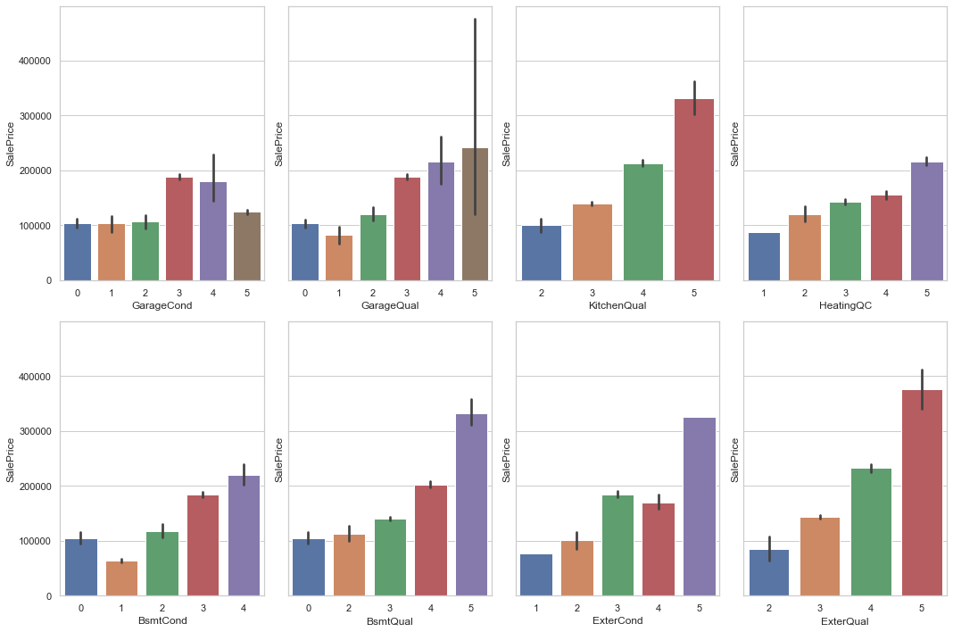
As you can see, the better the category of a variable, the higher the price, which means these variables will be important for a prediction model.
Nominal
Other categorical variables don't seem to follow any clear ordering.
Let's see how many values these columns can assume:
cols = train.columns
num_cols = train._get_numeric_data().columns
nom_cols = list(set(cols) - set(num_cols))
print(f'Nominal columns: {len(nom_cols)}')

value_counts = {}
for c in nom_cols:
    value_counts[c] = len(train[c].value_counts())

sorted_value_counts = {k: v for k, v in \
sorted(value_counts.items(), key=lambda item: item[1])}
sorted_value_counts
Nominal columns: 31
    {'CentralAir': 2,
     'Street': 2,
     'Utilities': 2,
     'LandSlope': 3,
     'PavedDrive': 3,
     'MasVnrType': 4,
     'GarageFinish': 4,
     'LotShape': 4,
     'LandContour': 4,
     'BsmtCond': 5,
     'MSZoning': 5,
     'Electrical': 5,
     'Heating': 5,
     'BldgType': 5,
     'BsmtExposure': 5,
     'LotConfig': 5,
     'Foundation': 6,
     'RoofStyle': 6,
     'SaleCondition': 6,
     'BsmtFinType2': 7,
     'Functional': 7,
     'GarageType': 7,
     'BsmtFinType1': 7,
     'RoofMatl': 7,
     'HouseStyle': 8,
     'Condition2': 8,
     'SaleType': 9,
     'Condition1': 9,
     'Exterior1st': 15,
     'Exterior2nd': 16,
     'Neighborhood': 25}
Some categorical variables can assume several different values like Neighborhood.
To simplify, let's analyze only variables with 6 different values or less.
nom_cols_less_than_6 = []
for c in nom_cols:
    n_values = len(train[c].value_counts())
    if n_values < 7:
        nom_cols_less_than_6.append(c)

print(f'Nominal columns with less than 6 values: \
{len(nom_cols_less_than_6)}')
Nominal columns with less than 6 values: 19
Plotting against SalePrice to have a better idea of how they affect it:
ncols = 3
nrows = math.ceil(len(nom_cols_less_than_6) / ncols)
f, axes = plt.subplots(nrows, ncols, figsize=(15, 30))

for r in range(0, nrows):
    for c in range(0, ncols):
        if not nom_cols_less_than_6:
            continue
        sns.barplot(x=nom_cols_less_than_6.pop(), \
        y="SalePrice", data=train, ax=axes[r][c])

plt.tight_layout()
plt.show()
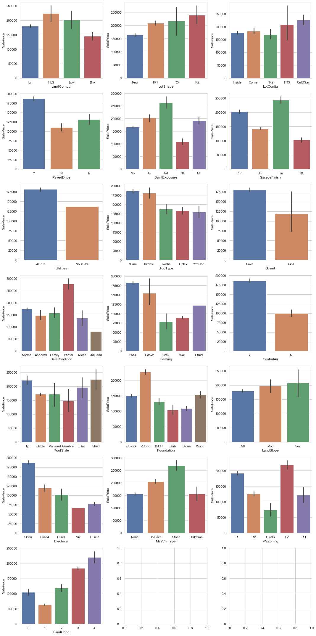
We can see a good correlation of many of these columns with the target variable.
For now, let's keep them.
We still have NaN in 'Electrical'.
As we could see in the plot above, 'SBrkr' is the most frequent value in 'Electrical'.
Let's use this value to replace NaN in Electrical.
# Inputs more frequent value in place of NaN

train['Electrical'].fillna('SBrkr', inplace=True)
Zero values
Another quick check is to see how many columns have lots of data equals to 0.
train.isin([0]).sum().sort_values(ascending=False).head(25)
    PoolArea         1164
    LowQualFinSF     1148
    3SsnPorch        1148
    MiscVal          1131
    BsmtHalfBath     1097
    ScreenPorch      1079
    BsmtFinSF2       1033
    EnclosedPorch    1007
    HalfBath          727
    BsmtFullBath      686
    2ndFlrSF          655
    WoodDeckSF        610
    Fireplaces        551
    FireplaceQu       551
    OpenPorchSF       534
    BsmtFinSF1        382
    BsmtUnfSF          98
    GarageCars         69
    GarageArea         69
    GarageCond         69
    GarageQual         69
    TotalBsmtSF        30
    BsmtCond           30
    BsmtQual           30
    FullBath            8
    dtype: int64
In this case, even though there are many 0's, they have meaning.
For instance, PoolArea (Pool area in square feet) equals 0 means that the house doesn't have any pool area.
This is important information correlated to the house and thus, we are going to keep them.
Outliers
We can also take a look at the outliers in the numeric variables.
# Get only numerical columns
numerical_columns = \
list(train.dtypes[train.dtypes == 'int64'].index)

len(numerical_columns)
42
# Create the plot grid
rows = 7
columns = 6

fig, axes = plt.subplots(rows,columns, figsize=(30,30))

x, y = 0, 0

for i, column in enumerate(numerical_columns):
    sns.boxplot(x=train[column], ax=axes[x, y])

    if y < columns-1:
        y += 1
    elif y == columns-1:
        x += 1
        y = 0
    else:
        y += 1

There are a lot of outliers in the dataset.
But, if we check the data description file, we see that, actually, some numerical variables, are categorical variables that were saved (codified) as numbers.
So, some of these data points that seem to be outliers are, actually, categorical data with only one example of some category.
Let's keep these outliers.
Saving cleaned data
Let's see how the cleaned data looks like and how many columns we have left.
We have no more missing values:
columns_with_miss = train.isna().sum()
columns_with_miss = columns_with_miss[columns_with_miss!=0]
print(f'Columns with missing values: {len(columns_with_miss)}')
columns_with_miss.sort_values(ascending=False)
    Columns with missing values: 0

    Series([], dtype: int64)
After cleaning the data, we are left with 73 columns out of the initial 81.
train.shape
(1168, 73)
Let's take a look at the first 3 records of the cleaned data.
train.head(3).T
| 0 | 1 | 2 | |
|---|---|---|---|
| MSSubClass | 20 | 60 | 30 |
| MSZoning | RL | RL | RM |
| LotArea | 8414 | 12256 | 8960 |
| Street | Pave | Pave | Pave |
| LotShape | Reg | IR1 | Reg |
| ... | ... | ... | ... |
| MoSold | 2 | 4 | 3 |
| YrSold | 2006 | 2010 | 2010 |
| SaleType | WD | WD | WD |
| SaleCondition | Normal | Normal | Normal |
| SalePrice | 154500 | 325000 | 115000 |
73 rows × 3 columns
We can see a summary of the data showing that, for all the 1168 records, there isn't a single missing (null) value.
train.info()
    <class 'pandas.core.frame.DataFrame'>
    RangeIndex: 1168 entries, 0 to 1167
    Data columns (total 73 columns):
    MSSubClass       1168 non-null int64
    MSZoning         1168 non-null object
    LotArea          1168 non-null int64
    Street           1168 non-null object
    LotShape         1168 non-null object
    LandContour      1168 non-null object
    Utilities        1168 non-null object
    LotConfig        1168 non-null object
    LandSlope        1168 non-null object
    Neighborhood     1168 non-null object
    Condition1       1168 non-null object
    Condition2       1168 non-null object
    BldgType         1168 non-null object
    HouseStyle       1168 non-null object
    OverallQual      1168 non-null int64
    OverallCond      1168 non-null int64
    YearBuilt        1168 non-null int64
    YearRemodAdd     1168 non-null int64
    RoofStyle        1168 non-null object
    RoofMatl         1168 non-null object
    Exterior1st      1168 non-null object
    Exterior2nd      1168 non-null object
    MasVnrType       1168 non-null object
    ExterQual        1168 non-null int64
    ExterCond        1168 non-null int64
    Foundation       1168 non-null object
    BsmtQual         1168 non-null int64
    BsmtCond         1168 non-null object
    BsmtExposure     1168 non-null object
    BsmtFinType1     1168 non-null object
    BsmtFinSF1       1168 non-null int64
    BsmtFinType2     1168 non-null object
    BsmtFinSF2       1168 non-null int64
    BsmtUnfSF        1168 non-null int64
    TotalBsmtSF      1168 non-null int64
    Heating          1168 non-null object
    HeatingQC        1168 non-null int64
    CentralAir       1168 non-null object
    Electrical       1168 non-null object
    1stFlrSF         1168 non-null int64
    2ndFlrSF         1168 non-null int64
    LowQualFinSF     1168 non-null int64
    GrLivArea        1168 non-null int64
    BsmtFullBath     1168 non-null int64
    BsmtHalfBath     1168 non-null int64
    FullBath         1168 non-null int64
    HalfBath         1168 non-null int64
    BedroomAbvGr     1168 non-null int64
    KitchenAbvGr     1168 non-null int64
    KitchenQual      1168 non-null int64
    TotRmsAbvGrd     1168 non-null int64
    Functional       1168 non-null object
    Fireplaces       1168 non-null int64
    FireplaceQu      1168 non-null int64
    GarageType       1168 non-null object
    GarageFinish     1168 non-null object
    GarageCars       1168 non-null int64
    GarageArea       1168 non-null int64
    GarageQual       1168 non-null int64
    GarageCond       1168 non-null int64
    PavedDrive       1168 non-null object
    WoodDeckSF       1168 non-null int64
    OpenPorchSF      1168 non-null int64
    EnclosedPorch    1168 non-null int64
    3SsnPorch        1168 non-null int64
    ScreenPorch      1168 non-null int64
    PoolArea         1168 non-null int64
    MiscVal          1168 non-null int64
    MoSold           1168 non-null int64
    YrSold           1168 non-null int64
    SaleType         1168 non-null object
    SaleCondition    1168 non-null object
    SalePrice        1168 non-null int64
    dtypes: int64(42), object(31)
    memory usage: 666.2+ KB
Finally, let's save the cleaned data in a separate file.
train.to_csv('train-cleaned.csv')
Summary of the EDA
We dealt with missing values and removed the following columns: 'Id', 'PoolQC', 'MiscFeature', 'Alley', 'Fence', 'LotFrontage', 'GarageYrBlt', 'MasVnrArea'.
We also:
- Replaced the NaN with NA in the following columns: 'GarageType', 'GarageFinish', 'BsmtFinType2', 'BsmtExposure', 'BsmtFinType1'.
- Replaced the NaN with None in 'MasVnrType'.
- Imputed the most frequent value in place of NaN in 'Electrical'.
Please note that the removed columns are not useless and may contribute to the final model.
After the first round of analysis and testing of the hypothesis, if you ever need to improve your future model further, you can consider reevaluating these columns and understand them better to see how they fit into the problem.
Data Analysis and Machine Learning is NOT a straight path.
It is a process where you iterate and keep testing ideas until you have the result you want, or until find out the result you need is not possible.
We are going to use this data to create our Machine Learning model and predict the house prices in the next post of this series.
Data Cleaning Script
This chapter converts the final decisions made to clean the data in the Exploratory Data Analysis into a single Python script that will take the data in CSV format and write the cleaned data also as a CSV.
Code
You can save the script on a file 'data_cleaning.py' and execute it directly with python3 data_cleaning.py or python data_cleaning.py, depending on your installation.
The script expects the 'raw_data.csv'.
The output will be a file named 'cleaned_data.csv'.
It will also print the shape of the original data and the shape of the new cleaned data.
Original Data: (1168, 81)
After Cleaning: (1168, 73)
The cleaning script:
import os
import pandas as pd

# writes the output on 'cleaned_data.csv' by default
def clean_data(df, output_file='cleaned_data.csv'):

    # Removes columns with missing values issues
    cols_to_be_removed = ['Id', 'PoolQC', 'MiscFeature', \
    'Alley', 'Fence', 'LotFrontage',
    'GarageYrBlt', 'MasVnrArea']
    df.drop(columns=cols_to_be_removed, inplace=True)

    # Transforms ordinal columns to numerical
    ordinal_cols = ['FireplaceQu', 'ExterQual', 'ExterCond', \
     'BsmtQual', 'BsmtCond',
    'HeatingQC', 'KitchenQual', 'GarageQual', 'GarageCond']
    for col in ordinal_cols:
        df[col].fillna(0, inplace=True)
        df[col].replace({'Po': 1, 'Fa': 2, 'TA': 3, \
        'Gd': 4, 'Ex': 5}, inplace=True)

    # Replace the NaN with NA
    for c in ['GarageType', 'GarageFinish', \
     'BsmtFinType2', 'BsmtExposure', 'BsmtFinType1']:
        df[c].fillna('NA', inplace=True)

    # Replace the NaN with None
    df['MasVnrType'].fillna('None', inplace=True)

    # Imputes with most frequent value
    df['Electrical'].fillna('SBrkr', inplace=True)

    # Saves a copy
    cleaned_data = os.path.join(output_file)
    df.to_csv(cleaned_data)

    return df

if __name__ == "__main__":
    # Reads the file train.csv
    train_file = os.path.join('train.csv')

    if os.path.exists(train_file):
        df = pd.read_csv(train_file)
        print(f'Original Data: {df.shape}')
        cleaned_df = clean_data(df)
        print(f'After Cleaning: {cleaned_df.shape}')
    else:
        print(f'File not found {train_file}')
How to Build the Machine Learning Model
Now we are going to use the 'cleaned_data.csv' file generated with the data cleaning script to generate the Machine Learning Model.
Train the Machine Learning Model
You can save the script in the file train_model.py and execute it directly with python3 train_model.py or python train_model.py, depending on your installation.
It expects you to have a file called 'cleaned_data.csv'.
The script will output three other files:
- model.pkl: the model in binary format generated by pickle that we can reuse later
- train.csv: the train data after the split of the original data into train and test
- test.csv: the test data after the split of the original data into train and test
The output on the terminal will be similar to this:
Train data for modeling: (934, 74)
Test data for predictions: (234, 74)
Training the model ...
Testing the model ...
Average Price Test: 175652.0128205128
RMSE: 10552.188828855931
Model saved at model.pkl
This means that the models used 934 data point to train and 234 data points to test.
The average Sale Price in the test set is $175,000.
The RMSE (root-mean-square error) is a good metric to understand the output because you can read it using the same scale as your dependent variable, which is Sale Price in this case.
A RMSE of 10552 means that, on average, we missed the correct Sale Prices by a bit over 10k dollars.
Considering an average of 175k, missing the mark by 10k on average is not too bad.
The Training Script
import numpy as np
import pandas as pd
from sklearn.preprocessing import OneHotEncoder
from sklearn.metrics import mean_squared_error
from sklearn.linear_model import LinearRegression
from sklearn.pipeline import Pipeline
import pickle


def create_train_test_data(dataset):
    # load and split the data
    data_train = dataset.sample(frac=0.8, \
    random_state=30).reset_index(drop=True)

    data_test = \
    dataset.drop(data_train.index).reset_index(drop=True)

    # save the data
    data_train.to_csv('train.csv', index=False)
    data_test.to_csv('test.csv', index=False)

    print(f"Train data for modeling: {data_train.shape}")
    print(f"Test data for predictions: {data_test.shape}")

def train_model(x_train, y_train):

    print("Training the model ...")

    model = Pipeline(steps=[
        ("label encoding", \
        OneHotEncoder(handle_unknown='ignore')),
        ("tree model", LinearRegression())
    ])
    model.fit(x_train, y_train)

    return model

def accuracy(model, x_test, y_test):
    print("Testing the model ...")
    predictions = model.predict(x_test)
    tree_mse = mean_squared_error(y_test, predictions)
    tree_rmse = np.sqrt(tree_mse)
    return tree_rmse

def export_model(model):
    # Save the model
    pkl_path = 'model.pkl'
    with open(pkl_path, 'wb') as file:
        pickle.dump(model, file)
        print(f"Model saved at {pkl_path}")

def main():
    # Load the whole data
    data = pd.read_csv('cleaned_data.csv', \
    keep_default_na=False, index_col=0)

    # Split train/test
    # Creates train.csv and test.csv
    create_train_test_data(data)

    # Loads the data for the model training
    train = pd.read_csv('train.csv', keep_default_na=False)
    x_train = train.drop(columns=['SalePrice'])
    y_train = train['SalePrice']

    # Loads the data for the model testing
    test = pd.read_csv('test.csv', keep_default_na=False)
    x_test = test.drop(columns=['SalePrice'])
    y_test = test['SalePrice']

    # Train and Test
    model = train_model(x_train, y_train)
    rmse_test = accuracy(model, x_test, y_test)

    print(f"Average Price Test: {y_test.mean()}")
    print(f"RMSE: {rmse_test}")

    # Save the model
    export_model(model)

if __name__ == '__main__':
    main()
The API
The output of the last chapter is the Machine Learning Model that we are going to use in the API.
Class HousePriceModel
Save this script in a file named predict.py.
This file has the class HousePriceModel and is used to load the Machine Learning model and make the predictions.
# the pickle lib is used to load the machine learning model
import pickle
import pandas as pd


class HousePriceModel():

    def __init__(self):
        self.model = self.load_model()
        self.preds = None

    def load_model(self):
        # uses the file model.pkl
        pkl_filename = 'model.pkl'

        try:
            with open(pkl_filename, 'rb') as file:
                pickle_model = pickle.load(file)
        except:
            print(f'Error loading the model at {pkl_filename}')
            return None

        return pickle_model

    def predict(self, data):

        if not isinstance(data, pd.DataFrame):
            data = pd.DataFrame(data, index=[0])

        # makes the predictions using the loaded model
        self.preds = self.model.predict(data)
        return self.preds
Create the API with FastAPI
To run the API:
uvicorn api:app
Here is the expected output:
INFO:     Started server process [56652]
INFO:     Waiting for application startup.
INFO:     Application startup complete.
INFO:     Uvicorn running on http://127.0.0.1:8000 (Press CTRL+C to quit)
The API is created with the framework FastAPI.
The "/predict" endpoint will give you a prediction based on a sample.
from fastapi import FastAPI
from datetime import datetime
from predict import HousePriceModel

app = FastAPI()

@app.get("/")
def root():
    return {"status": "online"}

@app.post("/predict")
def predict(inputs: dict):

    model = HousePriceModel()

    start = datetime.today()
    pred = model.predict(inputs)[0]
    dur = (datetime.today() - start).total_seconds()

    return pred
Testing the API
You can save the script in the file test_api.py and execute it directly with python3 test_api.py or python test_api.py, depending on your installation.
Remember to execute this test on a second terminal while the first one runs the server for the actual API.
Here's the expected output:
The actual Sale Price: 109000
The predicted Sale Price: 109000.01144237864
And here's the code to test the API:
# import requests library to make API calls
import requests
from predict import HousePriceModel

# a sample input with all the features we
# used to train the model
sample_input = {'MSSubClass': 20, 'MSZoning': 'RL',
'LotArea': 7922, 'Street': 'Pave',
'LotShape': 'Reg', 'LandContour': 'Lvl',
'Utilities': 'AllPub', 'LotConfig': 'Inside',
'LandSlope': 'Gtl', 'Neighborhood': 'NAmes',
'Condition1': 'Norm', 'Condition2': 'Norm',
'BldgType': '1Fam', 'HouseStyle': '1Story',
'OverallQual': 5, 'OverallCond': 7,
'YearBuilt': 1953, 'YearRemodAdd': 2007,
'RoofStyle': 'Gable', 'RoofMatl': 'CompShg',
'Exterior1st': 'VinylSd', 'Exterior2nd': 'VinylSd',
'MasVnrType': 'None', 'ExterQual': 3,
'ExterCond': 4, 'Foundation': 'CBlock',
'BsmtQual': 3, 'BsmtCond': 3,
'BsmtExposure': 'No', 'BsmtFinType1': 'GLQ',
'BsmtFinSF1': 731, 'BsmtFinType2': 'Unf',
'BsmtFinSF2': 0, 'BsmtUnfSF': 326,
'TotalBsmtSF': 1057, 'Heating': 'GasA',
'HeatingQC': 3, 'CentralAir': 'Y',
'Electrical': 'SBrkr', '1stFlrSF': 1057,
'2ndFlrSF': 0, 'LowQualFinSF': 0,
'GrLivArea': 1057, 'BsmtFullBath': 1,
'BsmtHalfBath': 0, 'FullBath': 1,
'HalfBath': 0, 'BedroomAbvGr': 3,
'KitchenAbvGr': 1, 'KitchenQual': 4,
'TotRmsAbvGrd': 5, 'Functional': 'Typ',
'Fireplaces': 0, 'FireplaceQu': 0,
'GarageType': 'Detchd', 'GarageFinish': 'Unf',
'GarageCars': 1, 'GarageArea': 246,
'GarageQual': 3, 'GarageCond': 3,
'PavedDrive': 'Y', 'WoodDeckSF': 0,
'OpenPorchSF': 52, 'EnclosedPorch': 0,
'3SsnPorch': 0, 'ScreenPorch': 0,
'PoolArea': 0, 'MiscVal': 0, 'MoSold': 1,
'YrSold': 2010, 'SaleType': 'WD',
'SaleCondition': 'Abnorml'}

def run_prediction_from_sample():

    url="http://127.0.0.1:8000/predict"
    headers = {"Content-Type": "application/json", \
    "Accept":"text/plain"}

    response = requests.post(url, headers=headers, \
    json=sample_input)
    print("The actual Sale Price: 109000")
    print(f"The predicted Sale Price: {response.text}")


if __name__ == "__main__":
    run_prediction_from_sample()
Conclusion
That's it!
Congratulations on reaching the end.
I want to thank you for reading this article.
If you want to learn more, checkout my blog renanmf.com.
You can also find me on Twitter: @renanmouraf.