

Artificial Intelligence is being used everywhere these days. And many of the groundbreaking applications come from Machine Learning, a subfield of AI.
Within Machine Learning, a field called Deep Learning represents one of the main areas of research. It is from Deep Learning that most new, truly effective AI systems are born.
But typically, the AI systems born from Deep Learning are quite narrow, focused systems. They can outperform humans in one very specific area for which they were made.
Because of this, many new developments in AI come from specialized systems or a combination of systems working together.
One of the bigger problems in the field of Deep Learning models is their lack of interpretability. Interpretability means understanding how decisions are made.
This is a big problem that has its own field, called explainable AI. This is the field within AI that focuses on making an AI model's decisions more easily understandable.
Here's what we'll cover in this article:
- Artificial Intelligence and the Rise of Deep Learning
- A big problem in deep learning: Lack of interpretability
- A solution to interpretability: Glass Box models
- Code example: Solving the problem with Explainable AI
- Conclusion: KAN (Kolmogorov–Arnold Networks)
This article won't cover dropout or other regularization techniques, hyperparameter optimization, complex architectures like CNNs, or detailed differences in gradient descent variants.
We'll just discuss the basics of deep learning, the lack of interpretability problem, and a code example.
Artificial Intelligence and the Rise of Deep Learning
 Photo by Tara Winstead
What is Deep Learning in Artificial Intelligence?
Deep Learning is a subfield of artificial intelligence. It uses neural networks to process complex patterns, just like the strategies a sports team uses to win a match.
The bigger the neural network, the more capable it is of doing awesome things – like ChatGPT, for example, which uses natural language processing to answer questions and interact with users.
To truly understand the basics of neural networks – what every single AI model has in common that enables it to work – we need to understand activation layers.
Deep Learning = Training Neural Networks
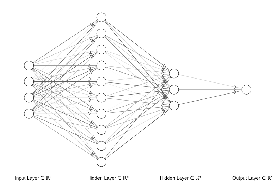 Simple neural network
At the core of deep learning is the training of neural networks.
That means basically using data to get the right values of each neuron to be able to predict what we want.
Neural networks are made of neurons organized in layers. Each layer extracts unique features from the data.
This layered structure allows deep learning models to analyze and interpret complex data.
A Big Problem in Deep Learning: Lack of Interpretability
 _Photo by Koshevaya_k_
Deep Learning has revolutionized many fields by achieving great results in very complex tasks.
However, there is a big problem: the lack of interpretability
While it is true that neural networks can perform every well, we don't understand internally how neural networks can achieve great results.
In other words, we know they do very well with the tasks we give them, but not how they do them in detail.
It is important to know how the model thinks in fields such as healthcare and autonomous driving.
By understanding how a model thinks, we can be more confident in its reliability in certain critical areas.
So models that work in fields with strict regulations are more transparent to the law and build more trust when they're interpretable.
Models that allow interpretability are called glass box models. On the other hand, models that do not have this capability (that is, most of them) are called black box models.
A Solution to Interpretability: Glass Box Models
Glass Box Models
 Photo by Pixabay: https://www.pexels.com/photo/fluid-pouring-in-pint-glass-416528/
Glass box models are machine learning models designed to be easily understood by humans.
Glass box models provide clear insights into how they make their decisions.
This transparency in the decision-making process is important for trust, compliance, and improvement.
Below we will see a code example of an AI model that, based on a dataset to predict breast cancer, it achieves an accuracy of 97%.
We'll also find, based on the characteristics of the data, which were of greater importance in predicting the cancer.
Black Box Models
In addition to glass box models, there are also black box models.
These models are essentially different neural network architectures used in various datasets. Some examples are:
- CNN (Convolutional Neural Networks): Designed specifically for image classification and interpretation.
- RNN (Recurrent Neural Networks) and LSTM (Long Short Term Memory): Primarily used for sequential data – text and time series data. In 2017, they were surpassed by a neural network architecture called transformers in a paper called Attention is All You Need.
- Transformer-based architectures: Revolutionized AI in 2017 due to their ability to handle sequential data more efficiently. RNN and LSTM have limited capabilities in this regard.
Nowadays, most models that process text are transformer-based models.
For instance, in ChatGPT, GPT stands for Generative Pre-trained Transformer, indicating a transformer neural network architecture that generates text.
All these models—CNN, RNN, LSTM and Transformers—are examples of narrow artificial intelligence (AI).
Achieving general intelligence, in my view, involves combining many of these narrow AI models to mimic human behavior.
Code Example: Solving the Problem with Explainable AI
 Photo by Chokniti Khongchum: https://www.pexels.com/photo/person-holding-laboratory-flask-2280571/
In this code example, we will create an interpretable AI model based on 30 characteristics.
We'll also learn what the 5 characteristics are that are more important in the detection of breast cancer, based on this dataset.
We will use a machine learning glass box model called the Explainable Boosting Machine
Here is the code below, which we will see block by block below:
import pandas as pd
from sklearn.model_selection import train_test_split
from sklearn.metrics import accuracy_score
from interpret.glassbox import ExplainableBoostingClassifier
import matplotlib.pyplot as plt
import numpy as np

# Load a sample dataset
from sklearn.datasets import load_breast_cancer
data = load_breast_cancer()
X = pd.DataFrame(data.data, columns=data.feature_names)
y = pd.Series(data.target)

# Split the data
X_train, X_test, y_train, y_test = train_test_split(X, y, test_size=0.2, random_state=42)

# Train an EBM model
ebm = ExplainableBoostingClassifier()
ebm.fit(X_train, y_train)

# Make predictions
y_pred = ebm.predict(X_test)
print(f"Accuracy: {accuracy_score(y_test, y_pred)}")

# Interpret the model
ebm_global = ebm.explain_global(name='EBM')

# Extract feature importances
feature_names = ebm_global.data()['names']
importances = ebm_global.data()['scores']

# Sort features by importance
sorted_idx = np.argsort(importances)
sorted_feature_names = np.array(feature_names)[sorted_idx]
sorted_importances = np.array(importances)[sorted_idx]

# Increase spacing between the feature names
y_positions = np.arange(len(sorted_feature_names)) * 1.5  # Increase multiplier for more space

# Plot feature importances
plt.figure(figsize=(12, 14))  # Increase figure height if necessary
plt.barh(y_positions, sorted_importances, color='skyblue', align='center')
plt.yticks(y_positions, sorted_feature_names)
plt.xlabel('Importance')
plt.title('Feature Importances from Explainable Boosting Classifier')
plt.gca().invert_yaxis()

# Adjust spacing
plt.subplots_adjust(left=0.3, right=0.95, top=0.95, bottom=0.08)  # Fine-tune the margins if needed

plt.show()
 Full Code
Alright, now let's break it down.
Importing Libraries
First, we'll import the libraries we need for our example. You can do that with the following code:
import pandas as pd
from sklearn.model_selection import train_test_split
from sklearn.metrics import accuracy_score
from interpret.glassbox import ExplainableBoostingClassifier
import matplotlib.pyplot as plt
import numpy as np
 Importing libraries
These are the libraries we are going to use:
- Pandas: This is a Python library used for data manipulation and analysis.
- sklearn: The scikit-learn library is used to implement machine learning algorithms. We're importing it for data pre processing and model evaluation.
- Interpret: The interpretAI Python library is what we'll use to import the model we'll use.
- Matplotlib: A Python library used to make graphs in Python.
- Numpy: Used for very fast numerical computations.
Loading, Preparing the Dataset, and Splitting the Data
# Load a sample dataset
from sklearn.datasets import load_breast_cancer
data = load_breast_cancer()
X = pd.DataFrame(data.data, columns=data.feature_names)
y = pd.Series(data.target)

# Split the data
X_train, X_test, y_train, y_test = train_test_split(X, y, test_size=0.2, random_state=42)
 Loading, Preparing the Dataset, and Splitting the Data
First, we load a sample dataset: We import a breast cancer dataset using the Interpret library.
Next, we prepare the data: The features (data points) from the dataset are organized into a table format, where each column is labeled with a specific feature name. The target outcomes (labels) from the dataset are stored separately.
Then we split the data into training and testing sets: The data is divided into two parts: one for training the model and one for testing the model. 80% of the data is used for training, while 20% is reserved for testing.
A specific random seed is set to ensure that the data split is consistent every time the code is run.
Quick note: In real life, the dataset is pre-processed with data manipulation techniques to make the AI model faster and to make it smaller.
Training the Model, Making Predictions, and Evaluating the Model
# Train an EBM model
ebm = ExplainableBoostingClassifier()
ebm.fit(X_train, y_train)

# Make predictions
y_pred = ebm.predict(X_test)
print(f"Accuracy: {accuracy_score(y_test, y_pred)}")
 Training the Model, Making Predictions and Evaluating the Model
First, we train an EBM model: We initialize an Explainable Boosting Machine model and then train it using the training data. In this step, with the data we have, we create the model.
This way, with one line of code, we create the AI model based on the dataset that will predict breast cancer.
Then we make our predictions: The trained EBM model is used to make predictions on the test data. Next, we calculate and print the accuracy of the model's predictions.
Interpreting the Model, Extracting, and Sorting Feature Importances
# Interpret the model
ebm_global = ebm.explain_global(name='EBM')

# Extract feature importances
feature_names = ebm_global.data()['names']
importances = ebm_global.data()['scores']

# Sort features by importance
sorted_idx = np.argsort(importances)
sorted_feature_names = np.array(feature_names)[sorted_idx]
sorted_importances = np.array(importances)[sorted_idx]
 Interpreting the Model, Extracting and Sorting Feature Importances
At this point, we need to interpret the model: The global explanation of the trained Explainable Boosting Machine (EBM) model is obtained, providing an overview of how the model makes decisions.
In this model, we conclude that the accuracy is approximately 0.9736842105263158 – which means the model is accurate 97 % of the time.
Of course, this only applies to the breast cancer data from this dataset – not for every single case of breast cancer detection. Since this is a sample, the dataset does not represent the full population of people seeking to detect breast cancer.
Quick note: In the real world, for classification, we'd use the F1 score instead of accuracy to predict how accurate a model is due to its consideration of both precision and recall.
Next, we extract feature importances: We extract the names and corresponding importance scores of the features used by the model from the global explanation.
Then we sort the features by importance: The features are sorted based on their importance scores, resulting in a list of feature names and their respective importance scores ordered from least to most important.
Plotting Feature Importances
# Increase spacing between the feature names
y_positions = np.arange(len(sorted_feature_names)) * 1.5  # Increase multiplier for more space

# Plot feature importances
plt.figure(figsize=(12, 14))  # Increase figure height if necessary
plt.barh(y_positions, sorted_importances, color='skyblue', align='center')
plt.yticks(y_positions, sorted_feature_names)
plt.xlabel('Importance')
plt.title('Feature Importances from Explainable Boosting Classifier')
plt.gca().invert_yaxis()

# Adjust spacing
plt.subplots_adjust(left=0.3, right=0.95, top=0.95, bottom=0.08)  # Fine-tune the margins if needed

plt.show()
 Plotting Feature Importances
Now we need to increase the spacing between feature names: The positions of the feature names on the y-axis are adjusted to increase the spacing between them.
Then we plot feature importances: A horizontal bar plot is created to visualize the feature importances. The plot's size is set to ensure it is clear and readable.
The bars represent the importance scores of the features, and the feature names are displayed along the y-axis.
The plot's x-axis is labeled "Importance," and the title "Feature Importances from Explainable Boosting Classifier" is added. The y-axis is inverted to have the most important features at the top.
Then we adjust the spacing: The margins around the plot are fine-tuned to ensure proper spacing and a neat appearance.
Finally, we display the olot: The plot is displayed to visualize the feature importances effectively.
The final result should look like this:
 Features importance graph
This way, we can conclude from an artificial intelligence model that is interpretable and has an accuracy of 97%, that the five most important factors in detecting breast tumors are:
- Worst concave points
- Worst texture
- Worst area
- Mean concave points
- Area error & worst concavity
Again, this is according to the provided dataset.
So according to the population that this sample dataset represents, we can conclude in a data-driven way that these factors are key indicators for breast cancer tumor detection.
This way, we can conclude from an artificial intelligence model, which methods interpret the model, that it provides clear insights into the significant features for prediction.
Conclusion: KAN (Kolmogorov–Arnold Networks)
Thanks to explainable AI, we can study populations using new data-driven methods.
Instead of only using traditional statistics, surveys, and manual data analysis, we can draw conclusions more accurately using an AI programming library and a database or Excel file.
But this is not the only way to have models built with explainable AI.
In April 2024, a paper called KAN: Kolmogorov–Arnold Networks was published that might shake up the field even more.
Kolmogorov–Arnold Networks (KANs) promise to be more accurate and easier to understand than traditional models and perform better.
They are also easier to visualize and interact with. So we'll see what happens with them.
You can find the full code here: